Within populations some people are very tall, while others are very short, with most people being somewhere in between. In other words, within populations there can be considerable variability in the height of individuals. This variability applies to other ‘populations’ as well. For example, if we weighed all the ‘1 kg’ (nominal weight) bags of sugar produced by two factories, A and B, we might find that although both manufacturing plants produce bags that weigh on average 1.010 kg, the bag weights for factory A might range from 0.981 kg to 1.061 kg, while those for factory B might only range from 1.001 kg to 1.021 kg. Therefore, while both factories are producing bags of sugar with the same average (mean) weight, it is quite clear that there is much greater variation in the weights of the bags of sugar produced by factory A compared with factory B – something that might be due to a lack of quality control in factory A.
From the illustration above, we can clearly see that if we want to describe the characteristics of any population, or sample taken from a population, it is not enough just to know the mean value, because we also need to know how much variability there is about the mean value. Statisticians have therefore developed several metrics: ‘sum of squares’; ‘variance’; and ‘standard deviation’, to quantify variability. These metrics, which are all closely related to each other, are summarized in Figure 1, which uses a small population (for illustrative purposes only) of twenty older adult subjects.
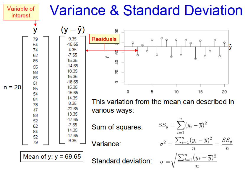
It can be observed from the example in Figure 1 that none of the subjects in the population has the same age as the mean value (i.e. 69.65 years). Some subjects are older and some are younger. In statistics the difference between mean value and the actual observed value, be it positive or negative, is known as the ‘residual error’, or ‘residual’ for short. Because some of these residuals are positive and some are negative, if we were to add them all together they would cancel each other out and we wouldn’t get a true picture of the variability in the population. Therefore, we square the residual for each individual before summing them all together, to produce the ‘sum of squares’, SSy, which for the example above is 4202.55 years. However, this is a rather unsatisfactory measure of variability because it is strongly influenced by the number of subjects in the population. Therefore, we divide the ‘sum of squares’ by the number of subjects, n, (in the case of a whole population) to produce the ‘variance’, σ2, which for the example above is 210.13 years. Although variance is a useful metric, it has the great disadvantage that it is based on the square of the residuals and so tends to be an order of magnitude greater than the mean value, making it difficult to interpret. We therefore square route the ‘variance’ to produce the ‘standard deviation’, σ, which is the variability metric most often used and is 14.50 years for the example above.
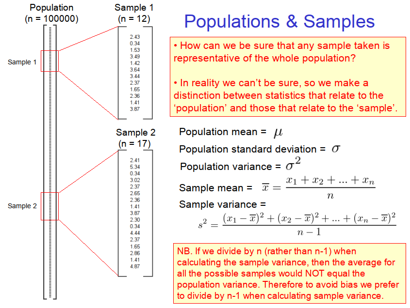
In the example above, we deliberately made the population small so that we could illustrate the concepts of variance and standard deviation. In reality, however, populations are often too large to measure and quantify, so we generally have to rely on smaller samples taken from larger populations. But how can we be sure that any sample that is taken is representative of the whole population? In reality we cannot be sure, so we need make a distinction between statistics that relate to the ‘population’ and those that relate to any given ‘sample’. Therefore, while we use μ, σ2 and σ to represent the mean, variance and standard deviation of populations, ͞x, s2 and s for the corresponding metrics in samples, as shown in Figure 2.
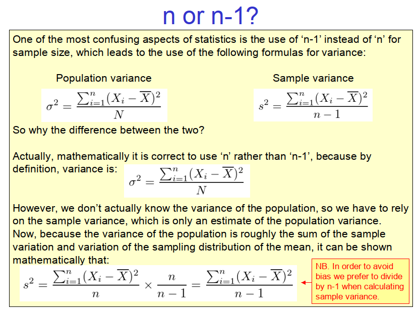
One rather strange ‘anomaly’ that often confuses students is that we use ‘n-1’ rather than ‘n’ when computing the variance and standard deviation of samples. Although it is mathematically correct to use ‘n’ rather than ‘n-1’, it is common practice to use ‘n-1’ in order to avoid any statistical bias (as explained in Figure 3).
Copyright: Clive Beggs