Before undertaking any statistical analysis, it is important first to understand the type of data that you are analysing, as this will strongly influence the selection of any statistical tests that you may wish to apply. Many statistical tests are only applicable to certain types of data and failure to recognise this fact can result in the wrong test being applied. For example, the chi-square test, which is often used to evaluate categorical data, should not be used with continuous data. Therefore it is important to recognise the differences between the various types of data that exist, as this will greatly help you when analysing data.
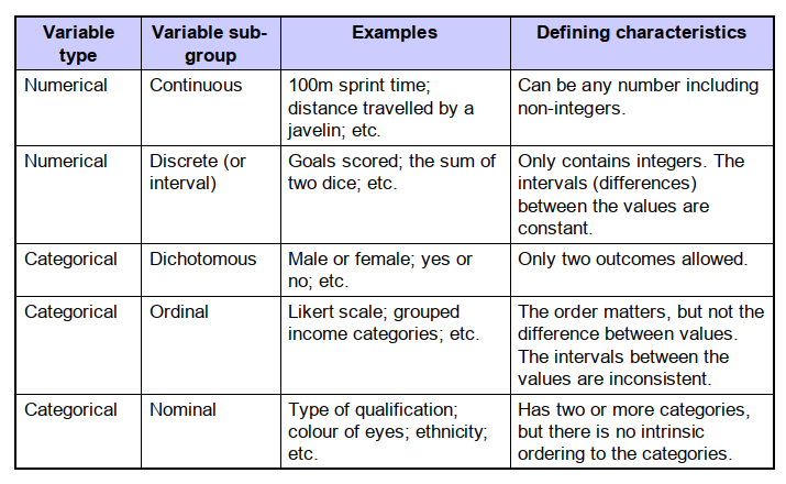
Broadly speaking data can classified as either being numeric or categorical. However, these broad classifications can be broken down into further sub-groups, as summarized in Table 1 below.
In order to expand on Table 1 and to illustrate the various types of data that you may encounter, let’s assume that we have designed a study with the aim of evaluating the differences in adult female populations from two countries, A and B. Let’s assume also that in the study we investigated 2000 age-matched adult female subjects, 1000 from country A and 1000 from country B, and that we collected various anatomical measurements from each subject. One measurement we might take, for example, is the subject’s height. This would result in a set of non-discrete decimal point measurements (e.g. 1.622 m, 1.718 m, 1.531 m, 1.832 m, etc.), which lie on a continuous scale and do not fit into any predefined categories. This type of data we define as a ‘continuous variable’ because each measurement collected can take any value on a continuous scale. Another measurement that we could acquire from the subjects is their dress size (e.g. 10, 12, 14, 16, 18, etc.). This is what is called a ‘discrete variable’ (or sometimes an ‘interval variable’), because the data has predefined discrete values, which are separated by a regular interval of known magnitude. While continuous and discrete variables are both numeric, it can be seen that the discrete variables comprise of whole numbers (i.e. integers), whereas continuous variables can contain decimal point numbers (i.e. non-integers). Importantly, however, despite this difference, it is possible with both types of variables to rank the data in order (e.g. short to tall, or small to large). This means that for both continuous and discrete variables it is possible to compute a mean (average) value, although how this should be interpreted in practise may be different for the two types of variable.
In addition to taking various measurements, we could also ask the subjects a set of research questions designed to acquire important information. At the simplest level, we could simply ask the women if they live in country A or B. This would elicit a response that was dichotomous, because there are only two answers to this question. Hence, the data acquired in response to this question would produce a ‘dichotomous variable’. Another question that we might ask is:
“In which sector do you work?”
This would yield responses that could be summarized in a contingency table, such as that shown in Table 2.
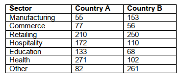
From Table 2 it can be seen that the data falls into discrete non-numerical categories, which were nominally predefined when the study was designed. Hence, this type of metric is called a catagorical variable. Importantly, however, there is no intrinsic order to these categories, so concepts like ‘mean value’ are meaningless with this type of data. All we can do is quantify the counts (frequencies) in each category. So for example, from Table 2 we can say that in country A more women appear to work in health than in manufacturing. We can also say that more women appear to work in manufacturing in country B compared with country A. Of course before we could be certain that this is the case, we would have to perform some sort of statistical analysis test, such as a chi-squared test.
Likert scales
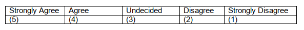
Another strategy that we could employ when soliciting information might be to use some predefined answers, in the form of a Likert scale, in response to questions or statements. So we could, for example, ask each subject:
“Do you enjoy going to work?”
To which they could be offered the following Likert scale from which to select one answer. (NB. Subjects select the appropriate number from 1 to 5 associated with their response.)

Note that although the response is categorical, unlike categorical variables, there is an order to the categories. Therefore, we call this type of data an ‘ordinal variable’. Note also, that unlike discrete variables, the intervals between the various responses are inconsistent and not of equal magnitude – the difference between ‘always’ and ‘often’ is not the same as that between ‘rarely’ and ‘never’. Consequently, because the intervals are inconsistent, great care must be taken when interpreting the mean score for this particular question. Indeed, with ordinal data, because the intervals between the data points are inconsistent or irregular, it is generally inadvisable to use the mean value. For this type of data the median and the mode are the only true measures of central tendency that can be used. Having said this, if the intervals can be made approximately equal (as outlined below), then the mean may also be of some value as an approximate measure of central tendency.
Because the intervals associated with ordinal variables can be uneven, this can present challenges when analyzing this type of data. Therefore, it is good practice to make the intervals as regular as possible, so that the mean score for the question can be used as an approximate measure of central tendency. This can be done by rephrasing the question in the form of a statement, as follows:
“I enjoy my job.”
We could then solicit a response using the following Likert scale, which has intervals of approximately even magnitude.
Now if we compute the mean score for this question, we are likely to get a answer that more closely reflects the true ‘average’ response for the study cohort.
Copyright: Clive Beggs