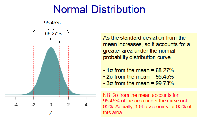
When we make random observations from populations in nature, we often find that the distribution of the sample conforms approximately to a normal (Guassian) distribution, such as that shown in Figure 1 below. This is because the populations themselves frequently exhibit a normal distribution, with most of the observations lying somewhere near the middle of the range and much fewer located at the extremities. Indeed, with a true normal distribution, 68.27% of the observations lie within one standard deviation of the mean and 95.45% within two standard deviations from the mean (as illustrated in Figure 1). This means that if we randomly select a value from the population, it is much more likely to come from the middle of the distribution than from its extremities. Therefore, if we randomly select samples from a population with a normal distribution, there is a higher probability that values near the centre of the distribution will be chosen.
Many ‘populations’ observed in biology, medicine and the social sciences exhibit normal distributions. As such, normality is an important concept in statistics. Indeed, the concept of normally lies at the heart of many statistical techniques. For example, parametric statistical techniques like Student’s t-test make the assumption that the sampling distribution of the mean (i.e. the distribution of the sample means as postulated by the central limit theorem (CLT)) is a normal distribution.
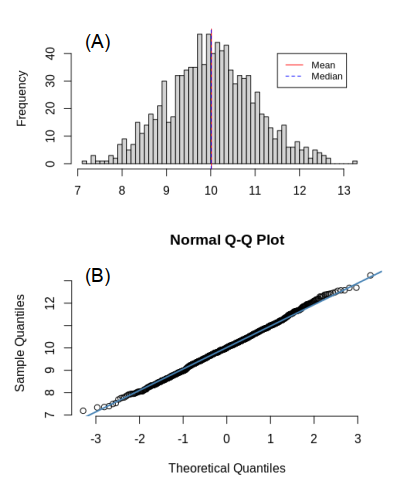
If we take a large enough random sample from a population with a normal distribution, we will find that the sample itself will be approximately normally distributed, with the mean and median values almost identical, as shown in Figure 2A. Moreover, if we produce a scatter plot by plotting the sample against a reference distribution that is normally distributed, the resultant quantile-quantile (QQ) plot will be a straight line (Figure 2B), revealing that a strong correlation exists between the sample and the reference distribution (i.e. indicating that the sample is normally distributed).
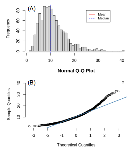
While many populations exhibit a normal distribution, it is not uncommon to encounter populations or samples that have a skewed distribution, such as that shown in Figure 3A. This is particularly the case when there is a cut-off threshold value, below (or above) which the observed values cannot fall (or rise). For example, if we consider the time spent in a waiting room by patients prior to seeing a doctor, the distribution of the waiting times will exhibit a skewed distribution. This is because the minimum waiting time is zero seconds (i.e. the lower threshold value). So while a minority of patients might have to wait for more than 30 minutes to see a doctor, none will wait less than zero seconds! Indeed, as can be seen in Figure 3A, most patients will be seen within 15 minutes, resulting in a distribution that is skewed to the right (i.e. it has a longer tail on the right-hand-side).
With skewed distributions the mean and the median values are not equal. If the distribution is skewed right, then the mean will be greater than the median value, whereas for a distribution that is skewed left, the relationship will be the other way round. The QQ plot for a sample with a skewed distribution will also be curved (as shown in Figure 3B), indicating that the sample is not normally distributed.
Testing for normality
While QQ plots can be useful for evaluating normality, they are not a statistical test per se. It is therefore advisable to use a statistical test such as the Shapiro–Wilk test to evaluate whether or not data are normally distributed. With the Shapiro-Wilk test the null-hypothesis is that the population is normally distributed. Thus, if p<0.05 we can reject the null hypothesis that the data are from a population that is normally distributed.
Skewness
The extent to which any given distribution is skewed can be evaluated using the Fisher-Pearson coefficient of skewness, g, which can be computed using the following formula.
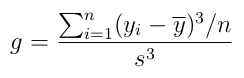
Where; yi is value of the ith item of data; ȳ is the mean; s is the standard deviation of the data; and n is the number of data points. (NB. When computing the skewness, s is computed using n as the denominator rather than n-1).
The skewness of any symmetrical data distribution, including a normal distribution is zero. A negative value for skewness indicates that the data distribution is skewed towards the left (i.e. the left tail is long compared with the right tail), while positive values indicate that data are skewed to the right.
Kurtosis
Like skewness, kurtosis is a statistical measure that can be used to describe the shape of a distribution. However, unlike skewness, which compares the weighting of the respective tails with each other, kurtosis measures the combined weight of a distribution’s tails relative to the centre of the distribution. For univariate data the formula for the kurtosis coefficient, k, is:
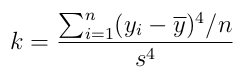
Where; yi is value of the ith item of data; ȳ is the mean; s is the standard deviation of the data; and n is the number of data points. (NB. When computing the skewness, s is computed using n as the denominator rather than n-1).
The kurtosis value for a normal distribution is 3, indicating that most of the data lies within ± 3 standard deviations of the mean. If the kurtosis <3, then this indicates that less data is contained in the tails compared with a normal distribution (i.e. the distribution has short tails), whereas if kurtosis>3 it indicates that the tails are longer than those for a normal distribution, suggesting that extreme values are more commonplace. As such, kurtosis can be considered a measure of the ‘tailedness’ of a distribution rather than its ‘peakedness’.
Copyright: Clive Beggs