Say we wanted to know whether or not a new training regime for athletes produced performance benefits. We could sample the running times of say 30 runners using the new training regime (i.e. the intervention group) and compare them to the times of say 40 runners trained using the old regime (i.e. the controls). While it would be easy for us to calculate the means and standard deviations of the two groups, how could we be sure that any observed difference in performance between the groups is actually representative of all runners, given the considerable variability in performance that naturally occurs between runners. In short, how can we be sure that the improvement in performance that we might observe in the experiment is actually due to the new training regime and not due to natural variability. After all, the observed improvement (the so-called ‘effect’) might simply be because we inadvertently put the fast runners in the intervention group and the slow runners in the control group, something that could happen just by chance!
Well the simple answer to the problem described above is that we cannot be absolutely (i.e. 100%) sure that our intervention has worked. All we can do, at best, is to say that we are very confident that the intervention has worked – statistics does not allow us to be 100% confident!
So how can we be confident whether or not any given intervention has been successful? Although this is a difficult question to answer, statisticians have come up with a robust methodology called ‘hypothesis testing’ that has proved to be extremely helpful and which is widely used by scientists around the world. In this tutorial we will investigate the concept of hypothesis testing because it is an important subject in statistics and one that is often misunderstood by students and researchers.
Example experimental study
To illustrate hypothesis testing, let us consider a hypothetical weight loss study designed to test the efficacy of a new diet. Let’s assume that we have a study cohort of 170 female subjects (all of a similar age) and that we are interested in assessing the impact of the new diet on weight loss over a six-month period. If we randomly divide the study cohort into two groups, a control group of say 80 subjects who do not change their diet, and an intervention group of say 90 subjects who follow the new diet, then we can compare the mean weights of the two groups at the end of the study in order to determine whether or not any weight loss (i.e. the effect) has occurred.
For illustrative purposes only, let us assume that the study can have one of two outcomes:
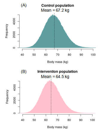
- Scenario 1 (termed the null hypothesis, H0): The diet has no effect and that both groups are effectively just samples taken from the same population, which has a mean of 67.2 kg.
- Scenario 2 (termed the alternative hypothesis, H1): The diet has been effective and the intervention group has actually lost weight, to such an extent that it can be considered to be a sample taken from a population which has a mean of 64.5 kg.
Note that in reality it would not be possible for us to specify the parameters of the respective populations for each outcome scenario, because they are not known. However, in order to illustrate the concepts of the null and alternative hypotheses it is helpful for us to do so here. Note also that we only have two outcomes:
- Scenario 1, where we accept the null hypothesis, H0, that the diet has had no effect.
- Scenario 2, where we reject the null hypothesis, H0, in favour of the alternative hypothesis, H1, that the diet has had an effect.
In statistics when we perform a hypothesis test the result is always one of these two outcomes, and we either reject or accept the null hypothesis. So actually it is the null hypothesis that we are testing!
Control and intervention populations
In reality body mass is not normally distributed in populations, but is actually slightly skewed to the right [1], approximating roughly to a gamma distribution. The respective control and intervention populations are shown in the histograms in Figure 1, which both have a gamma distribution and means of 67.2 kg and 64.5 kg respectively. Note that both populations have distributions that are slightly skewed towards the right. This is important, because it demonstrates that the populations themselves do not need to be normally distributed in order for hypothesis testing to be undertaken.
Null distribution
In order to illustrate the null hypothesis it is necessary first to introduce the concept of the ‘null distribution’. The null distribution in this case is the distribution of weight loss outcomes that might occur just by chance due to natural variability in the population, assuming that the intervention (i.e. the diet) has had no overall effect.
Before the advent of statistical computing, producing a null distribution was a difficult thing to do by hand. However, using R or Python it is a relatively simple task, using the following procedure.
- Take a random sample of 80 subjects from the control population. This will be our control group sample.
- Take a second random sample containing 90 subjects from the control population. This will be the intervention group sample.
- Compute the difference between the means of the two samples (i.e. compute the sample effect).
- Repeat this process 10000 times to produce the distribution of the sample effects. This distribution is the null distribution (i.e. the distribution that would occur by chance, assuming that the diet has had no effect on the weight of the subjects).
The resulting null distribution is shown in Figure 2, below.
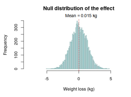
From Figure 2 it can be seen that the resulting null distribution ranges from approximately –5 kg to 5 kg, with a mean value of approximately 0 kg, which is what we would expect if no weight loss effect had occurred. Furthermore, the resulting null distribution is normally distributed, despite the fact that the control population was right skewed. This is because the central limit theoren (CLT) dictates that the distribution of the effect must be normal.
Alternative distribution
The alternative distribution, which is associated with the alternative hypothesis, can be produced using the same methodology as that for the null distribution, but with the alteration that the intervention samples (containing 90 subjects) are taken from the intervention population rather than the control population. If this is done, then the alternative distribution produced is as shown in Figure 3.
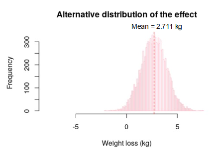
It can be observed from Figure 3 that the resulting alternative distribution is normally distributed with a mean of 2.711 kg, which is what we would expect if a weight loss effect had occurred.
Significance
If we now mimic the actual weight loss experiment by randomly selecting 80 subjects from the control population and 90 subjects from the intervention population (assuming that the alternative hypothesis is true), we might obtain the result that the diet produced a mean weight loss of 3.059 kg. While this might appear at first site to demonstrate that diet works, how can we be confident that this observed effect is not just a chance result arising purely from subject variability?
Well, if we plot the observed result (i.e. the effect) of 3.059 kg on both the null and alternative distributions (as shown in Figure 4), we can see that while it falls at the extreme end of the null distribution, it falls near the middle of the alternative distribution. This means that the observed result is much more likely to come from the alternative distribution than from the null distribution. Suggesting that we might be able to reject the null hypothesis. However, in reality while we can plot the null distribution, we cannot plot the alternative distribution, because we don’t know what it is. Therefore, we have to rely on the null distribution only, do determine whether or not our experimental result is ‘significant’ or not.
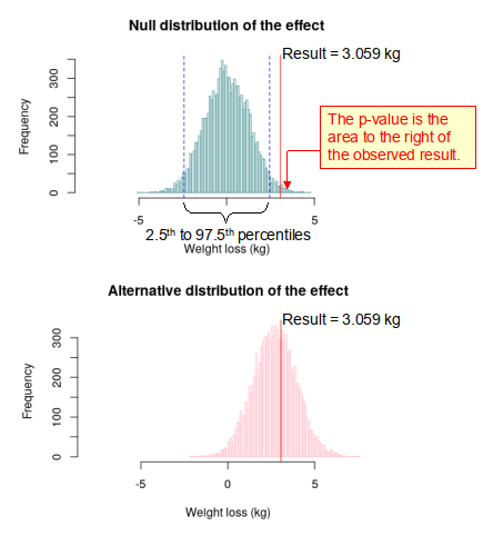
Fortunately, statisticians have developed a methodology, which requires only the null distribution to determine if an experimental result is statistically ‘significant’ (i.e. a result that we can be confident in) or not. For a two-tailed hypothesis test such as the weight loss study above (NB. it is two-tailed because we did not know the direction of the effect before hand), it is assumed that if the observed result lies in the tails of the null distribution, either less than the 2.5th percentile or greater than the 97.5th percentile, then the result probably belongs to an alternative distribution. In other words, if the observed result lies outside this range, as is the case in Figure 4, then we can safely reject the null hypothesis and accept the alternative hypothesis. When we reject the null hypothesis we say that the result is statistically significant.
p-value
As well as determining whether or not a test result is significant, it is also possible using the null distribution to determine the p-value. Quite simply, the p-value is the probability of obtaining a test result at least as extreme as the result actually observed during the test, assuming that the null hypothesis is correct [2]. Therefore, in the example above the p-value is simply the fraction of the area under the null distribution curve that lies to the right of the observed result. In Figure 4 it can be seen that on just 89 out of 10000 occasions was the figure of 3.059 kg either equalled or exceeded in the null distribution. Therefore, the p-value is 0.009 (something that is confirmed by an independent t-test).
References
- Hermanussen M, Danker-Hopfe H, Weber GW. Body weight and the shape of the natural distribution of weight, in very large samples of German, Austrian and Norwegian conscripts. International journal of obesity. 2001. 25: 1550.
- Wasserstein, Ronald L. ASA statement on statistical significance and P-values. The American Statistician. 2016. 70: 131-133
Copyright: Clive Beggs