The chi-squared test, first developed by Karl Pearson at the end of the 19th century, is a widely used technique for determining whether or not a statistically significant difference exists between the expected and observed frequency counts in one or more categories of contingency table. It is underpinned by a very simple idea, namely that if there is no difference between two classes (say Class A and Class B) in a population, then if we take a sample from that population we would expect to see both classes equally represented in the sample. So, if we toss a fair coin 100 times we would expect that it would land approximately 50 times as heads and approximately 50 times as tails. However, if it lands 90 times as heads and only 10 times as tails, then we might get suspicious that coin is not fair and that it is biased in some way.
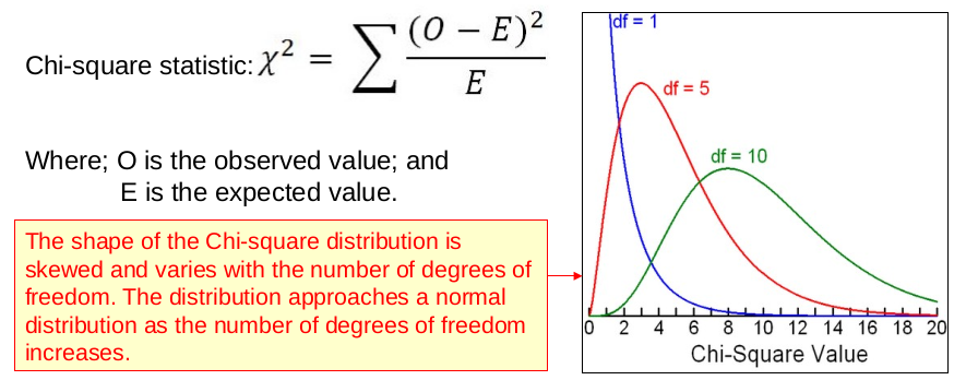
The chi-squared test is very useful when testing hypotheses which involve categorical (e.g. eye colour, etc.) or dichotomous (e.g. yes/no) data. This type of nominal data is generally analyzed by frequency of occurrence, with observations assigned to mutual exclusive categories, which categorize the various sub-groups within the data. With respect to this, the chi-squared statistic (see Figure 1) is used to compare relative frequency of occurrence over two or more groups.
Simple example
Imagine that we toss a coin 160 times and record the outcome. If the coin is fair we would expect it to land on heads for 50% of the tosses and on tails for 50% of the tosses. However, in our experiment we find that the coin landed heads on 86 occasions and tails on 74 occasions (see Figure 2). So is this a fair result (within the bounds of reasonable possibility), or is the coin loaded?
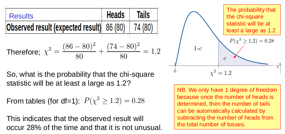
The contingency table in Figure 2, reveals that we would expect the coin to land 80 times as heads and 80 times as tails. From the this and the observed values we can compute the chi-squared statistic of 1.2, which when applied to a chi-squared probability distribution reveals that the result is not at all unusual. So, we can accept the null hypothesis and conclude that the coin is fair.
The chi-squared test is often used to test associations between variables in two-way tables, where the assumed model of independence (the null hypothesis) is evaluated against the observed data. In such circumstances, we set up a null hypothesis which assumes that no interactions take place and then calculate the values that we expect to occur if the null hypothesis were true. We then compare these expected values with the observed values as illustrated in the following example.
More complex example
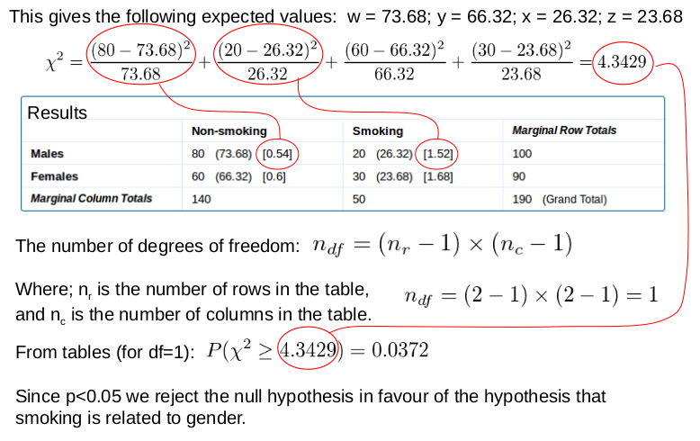
Suppose we want to find out whether or not smoking is related to gender. We therefore perform a study on the smoking habits of 100 male and 90 female adult subjects. The results of this study are presented in the [2 x 2] contingency table below.
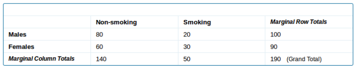
From this we can see that in this study more females smoked than males. But how can we be sure that this result has general applicability?
In order to perform the chi-squared test, we must first state the null hypothesis (H o), which is in this case is that ratio of smokers to non-smokers is the same for both males and females. If this hypothesis is correct then we would expect certain expected values w, x, y, and z in the four data positions in the table below:
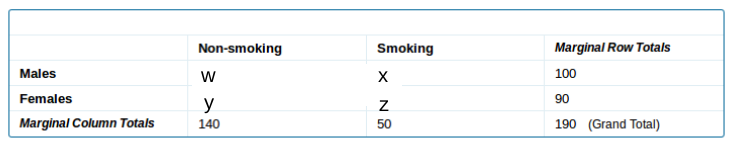
Because the null hypothesis is that the ratios are the same, then we must have:
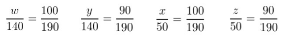
This gives the following expected values: w = 73.68; y = 66.32; x = 26.32; z = 23.68, which we can use to calculate the chi-squared value (i.e. 4.343).
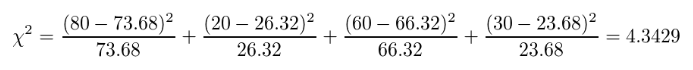
Figure 3 shows how the rest of the calculation is done by hand. From this, we can see that the observed ratios are very different between the males and females. Therefore, we can reject the null hypothesis (H o) (i.e. there is no difference) in favour of the alternative hypothesis (H 1) that there is a difference between the males and the females.
Copyright: Clive Beggs