It is often possible to establish whether or not a statistical difference exists between the results obtained from two groups by using a simple t-test. The t-test, first introduced in 1908 by William Sealy Gosset under the pen name ‘Student’ [1], is one the most widely used hypothesis testing techniques in statistics. However, Student’s original t-test has the great disadvantage that it requires the sample variances of the two groups to be equal, which is often not the case. So here we will explain Welch’s t-test, which is a variant of the t-test that performs better than Student’s version when the sample sizes and variances of the two groups are unequal. When comparing observations (results) that are independent of each other, Welch’s t-test is the superior test because it is more versatile and robust compared with Student’s t-test [2,3].
When we perform a t-test, we are actually testing the null hypothesis that the results (observations) for both groups are just samples taken from the same ‘population’ and that there is actually no real difference between the two groups (see here to find out more about hypothesis testing and the null hypothesis). At first sight, this might appear to be a ‘back-to-front’ approach to take. However, if we can show that the observed ‘effect’ (i.e. the difference between the means of the results for the two groups) is unlikely to have occurred by chance, then we can reject the null hypothesis and conclude that there is a real statistical difference between the two groups (i.e. accept the alternative hypothesis).
Paradoxically, the best way to understand the t-test is to first look at the two-sample Z-test, which is closely related to it. The two-sample Z-test uses the Z-score (see here for more information on Z-scores and p-values), which is based on a standardized normal distribution, whereas the t-test uses a modified normal distribution that takes into account the sample size. When sample sizes are small (i.e. n<30 observations), then the t-test gives superior results, whereas when n >=30 then the Z-test performs better. Having said this, the t-test and Z-test are virtually the same test when n >=30. When n >=30, the Z-score can be computed using the following equation, in which the numerator is the difference between the two means (i.e. the effect), and the denominator is the standard error of the difference between the means.
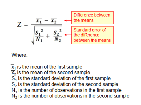
From this equation it can be seen that the Z-score is simply the ratio of the difference between the sample means, to the standard error of the difference between the means. Importantly, if the standard error is large, say because the sample size is small, then the Z-score will tend to be small and the test is unlikely to produce a significant result (i.e. p<0.05).
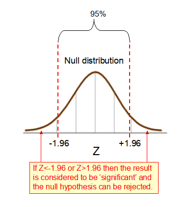
In the context of a 2-tailed hypothesis test, if the computed Z-score is <-1.96 or >1.96 (as shown in Figure 1 below), then we can reject the null hypothesis that there is no difference between the observed results for the two groups and instead accept the alternative hypothesis that the observed effect is real and not likely to have occurred by chance. When the Z-score falls outside this range we say that the p-value is statistically significant at a = 0.05 (see here for more details about p-values).
Welch’s independent t-test
In studies where the two samples are independent of each other (i.e. the subjects in the two groups are different) Welch’s t-test should be used. Welch’s t-test utilizes a metric, the t-statistic, which like the Z-score is the ratio of the difference between the means, to the standard error of the difference between the means. The t-statistic can be computed using the following equation, which is identical to that for the Z-score above.
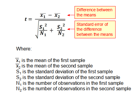
While the formula for computing the t-statistic is the same as that for the Z-score, how the two statistics are used is slightly different. With the Z-score, it is assumed that the null distribution of the effect (i.e. the difference between the means) is normally distributed, as dictated by the central limit theorem (CLT). However, this is only true if the sample sizes are relatively large, say n 30. When the sample sizes are smaller than this, as is often the case, then the null distribution conforms to a t-distribution, which is flatter and has longer tails than those found in the normal distribution. When sample sizes are small, if a normal distribution is wrongly assumed, this will lead to an underestimation of the variance of the null distribution. The t-distribution compensates for this underestimation by having thicker tails than the normal distribution. However, as the sample size (N) grows, so the t-distribution, which is characterized by the number of degrees of freedom (df), becomes more and more similar to a normal distribution, reflecting the fact that the sample variance more accurately reflects the variance of the population.
The t-distribution is used to evaluate the significance of the t-statistic, in a similar fashion to the Z-score. When N is small, the p-values derived from the t-distribution vary greatly as N changes. With Welch’s t-test the number of degrees of freedom, df, of the t-distribution can be computed using the Satterthwaite-Welch equation below.
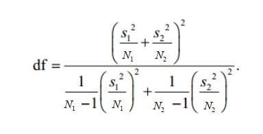
Where: N1 and N2 are the number of observations in the two samples; and S1 and S2 are the standard deviations of the respective samples.
Limitations of Welch’s t-test
Welch’s independent t-test is used to compare the means of two unrelated groups (i.e. the same subjects must not appear in both groups). It is limited to use with continuous numeric variables, and should not be used with categorical or ordinal variables.
It is often wrongly assumed that Welch’s t-test cannot be used when the data is not normally distributed. This is incorrect. The t-test assumes that the means of the different samples are normally distributed, not that populations themselves are normally distributed. Even when the measured samples come from populations that have a skewed distribution, because of the CLT, the sampling distribution of the means will have a normal distribution (see here for more details), provided that the sample size is large enough >=30. Therefore, Welch’s t-test remains robust for skewed distributions when sample sizes are large [3]. Having said this, reliability decreases for samples with skewed distributions, when sample sizes are small [4].
Paired t-test
When samples are not independent, because they are matched or paired, as is the case with say a ‘before and after intervention’ study, then a modified version of the t-test (see equation below) should be used known as a paired t-test.
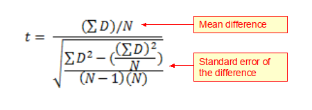
Where: N is the number of pairs of observations; and ΣD is the sum of all the respective differences.
The paired t-test should be used when the same subjects appear in both groups of interest, whereas when the subjects are different in the two groups an independent t-test should be used.
References
- Mankiewicz R. The story of mathematics. Cassell; 2000
- Zimmerman, D. W. A note on preliminary tests of equality of variances. British Journal of Mathematical and Statistical Psychology. 2004.57: 173–181.
- Fagerland, M. W. t-tests, non-parametric tests, and large studies—a paradox of statistical practice?. BMC Medical Research Methodology. 2012. 12: 78.
- Fagerland, M. W.; Sandvik, L. Performance of five two-sample location tests for skewed distributions with unequal variances. Contemporary Clinical Trials. 2009. 30 (5): 490–496.
Copyright: Clive Beggs