Although the central limit theorem (CLT) is one the most important concepts in statistics, most people either don’t understand it or have never heard of it. Yet it underpins some of the most widely used techniques in statistics, such as the t-test and ANOVA. So it is worth spending a few minutes to get a deeper understanding of the CLT and its importance in statistics.
The CLT simply states that if we take lots of samples of the same size from a population, then provided the samples are sufficiently large, the distribution of the means of the respective samples (also known as the sampling distribution of the mean) will be a normal distribution (assuming true random sampling), regardless of the distribution of the original population. Although this explanation of the CLT might appear obscure and irrelevant, it is in fact the reason why were can trust techniques like the t-test and ANOVA.
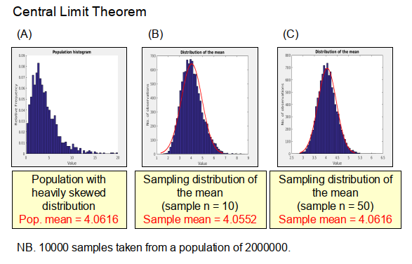
So lets look at an example of the CLT to get a better understanding of how it works. Consider the large hypothetical population shown in (A) of Figure 1, which has a mean of 4.062 and a distribution that is heavily skewed. If we take 10000 samples from this population, each with a sample size of 10, and then plot the distribution of the means of the individual samples (what we call the sampling distribution of the mean) as shown in Figure 1(B), we find rather surprisingly that it approximates to a normal distribution (i.e. the red line curve in Figure 1(B)) with an overall mean, in this case, of 4.055. If we then increase the sample size to 50 (see Figure 1(C)) and repeat the process again we find that a normal distribution is produced which has the same mean value as that of the overall population, which is exactly what the CTL predicts.
Because of the CLT it is possible to determine quite accurately the characteristics of a large population without having to actually measure the whole population. All we need to do is take a lot of samples of a reasonable size and then we can infer from these the mean and the standard deviation of the whole population. Polling companies do this all the time when they try to predict the outcome of elections.
Importantly, we don’t have to take that many samples to get a reasonable approximation of the mean of the population. For example, if we repeat the analysis above, but this time just taking 100 samples, we find that for a sample size of 10 the predicted mean is 3.898, and for a sample size of 50 it is 4.067, which is very close to the true population mean. Therefore, while we don’t have to take that many samples to get a good approximation of the mean, it is important to ensure that the sample size is large enough – generally greater than 30 is thought to be a good first approximation.
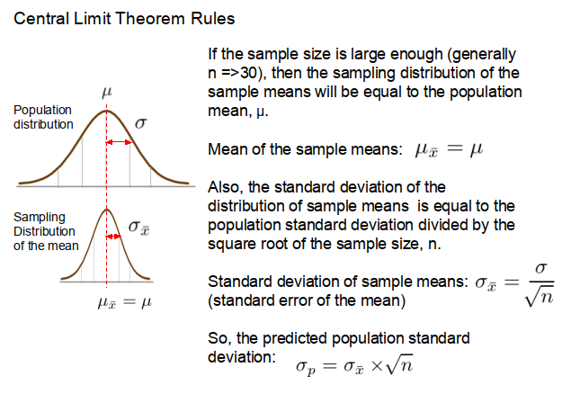
So how can we estimate the population mean and standard deviation from just a few samples? Well conveniently, if the sample size is large enough (i.e. 30 or greater), then the mean of the sample means, μ͞x, will be equal to the population mean, μ (see Figure 2). Also, the standard deviation of the distribution of the sample means, σ͞x, (otherwise known as the standard error of the mean) will conform to the following equation.

where: n is the sample size; and σ is the standard deviation of the population.
So, if the standard deviation of the distribution of the sample means is known it is easy to calculate the standard deviation of the whole population, as illustrated in the example below.
Example
Question:
Say that we want to estimate the mean and standard deviation of the age of a city’s population (4000000 inhabitants).
If we take 200 samples (each of size n = 30) and find the mean and standard deviation of the sample means is 33.5 years and 2.7 years respectively, what is the estimated mean and standard deviation of the population?
Answer:
The mean is same as the mean of the sample means (i.e. 33.5 years)
The estimated population standard deviation is: 2.7 ⨯√30 = 14.79 years
Copyright: Clive Beggs