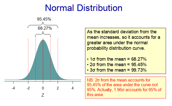
Many populations in biology, medicine and the social sciences exhibit a normal (Guassian) distribution, with most of the observations lying somewhere near the middle of the range, and much fewer located at the extremities. Indeed, with a true normal distribution, 68.27% of the observations lie within one standard deviation of the mean and 95.45% within two standard deviations from the mean (as illustrated in Figure 1).
Because normal distributions are frequently observed in nature, they form the basis of a whole branch of statistics, namely parametric statistics. Parametric statistical analysis assumes that sample data come from populations that can be modelled using a normal probability distribution that has a fixed set of parameters.
If we randomly select a value (observation) from a normally distributed population, it is much more likely to come from the middle of the distribution than from its extremities. Therefore, we can use a normal distribution curve to assess the probability (likelihood) of an event or observation occurring. So a normal distribution curve can be considered akin to a probability density curve, which can be generated using the following mathematical function.
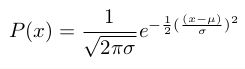
Where:
- P(x) is the probability of the value, x, occurring;
- x is any value of a continuous variable;
- μ is the mean of the population;
- σ is the standard deviation of the population;
- π is the mathematical constant 3.14159; and
- e is the mathematical constant 2.71828.
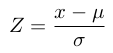
So, in theory, if we know the mean and the standard deviation of a population, we can generate the probability density function for that population and use this to assess the probability of any particular event or observation occurring. However this is a bit ‘messy’, because every normal distribution has a different mean value and standard deviation, making the calculation somewhat difficult. So statisticians came up with the idea of standardizing the normal distribution curve using a Z-score, which is a measure of how many standard deviations above or below the mean value an observed value, x, is. This is done by transforming the observed distribution, X, into a standardized normal distribution, Z, with μ = 0 and σ = 1.
The observed values, x, can easily be transformed into Z-scores using:
This creates the standardized normal distribution curve shown in Figure 1 above, which has a mean value of zero. Importantly, the area under the standardized curve is equal to one, something that is particularly helpful, when computing p-values from Z-scores, as we can see from the following example.
Example
Question:
Given that the female gestation period (i.e. the period between conception and birth) conforms to a normal distribution with a mean of 266 days and a standard deviation of 16 days, what is the probability that a pregnancy will last 294 days or longer?
Answer:
First, we need to convert the x value (i.e. 294 days) to a Z-score as follows:
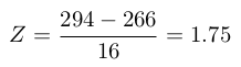
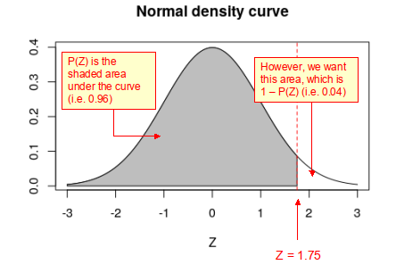
When this Z-score is plotted on the standard normal curve below it can be seen that area under the probability density curve to the left of the red dotted line (i.e. P(Z)) is 0.96. While that to the right of the red dotted line (i.e. 1 – P(Z)) is 0.04. This can be interpreted as the probability of the gestation period being <294 days is 0.96, whereas the probability (p-value) that it is >294 days is 0.04. That is 4% of pregnancies exceed a gestation period of 294 days.
Before the advent of statistical computing, in order to determine the area under the probability density curve it would be necessary to look-up a Z-score to p-value transformation table – a somewhat slow and tedious task. However, with R is it easy to convert from a Z-score to a p-value using just a few lines of code, as follows:
In R:
# Converting a Z-score to a p-value in Rz = 1.75 # This is the Z-scorepvalue = pnorm(-abs(z)) # This transforms the Z-score to a p-valueprint(1-pvalue) # The probability of less than the observed Z-scoreprint(pvalue) # The probability of greater or equal than the Z-score
One or two-tails?
Note that in the example above, we asked the question:
“What is the probability that a pregnancy will last 294 days or longer?”
This is what statisticians call a ‘one-tailed’ problem, because we asked the question in one direction only (i.e. “What is the probability of having an extremely long gestation period?”). We could however, have asked: “What is the probability of having either an extremely short or extremely long gestation period?” In which case, we are posing a ‘two-tailed’ problem, because the concerns extreme observations in both tails of the normal distribution curve.
p-values
Many people reading this webpage will of heard about p-values and will have a vague idea of what they are. However, if we asked them to explain exactly what a p-value is, they might struggle. Indeed, while p-values are widely quoted in the life and social sciences, surprisingly few people fully understand what they represent. In fact, the definition of a p-value in the context of hypothesis testing is:
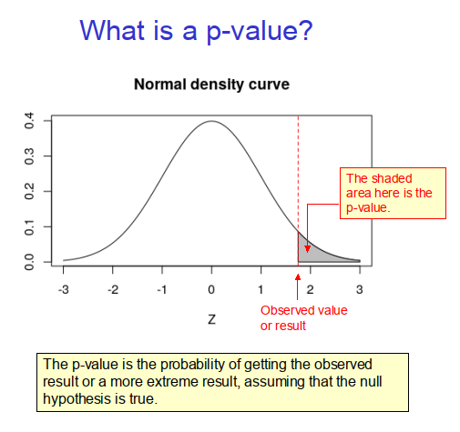
‘The p-value (or probability value) is the probability of obtaining test results at least as extreme as the result actually observed during the test, assuming that the null hypothesis is correct.’ [1]
In the context of the one-tailed example above the p-value is therefore 0.04, because this is the probability that the gestation period will be at least 294 days or longer, as illustrated in Figure 2 below.
References
- Wasserstein, Ronald L. ASA statement on statistical significance and P-values. The American Statistician. 2016. 70: 131-133.
Copyright: Clive Beggs